Introduction
We still have a limited understanding of how Large Language Models (LLMs) achieve impressive results across a wide array of tasks (Devlin et al. 2019; Grattafiori et al. 2024). While a growing body of work interprets LLMs using behavioural experiments, probing, or causal interventions, the scale of these models makes understanding how their representation spaces are structured a continued challenge. Here we look at an LLM as an instance of lossy compression, offering an account of how models represent information during training and what information matters for performance.
Lossy compression represents data efficiently by preserving only the information from a source relevant to a goal. While audio recordings intended for human listeners can be gigabytes in size, MP3 files save space by discarding frequencies typically outside the range of human hearing (Jayant, Johnston, and Safranek 1993); similarly, a JPEG file omits subtle colour variations that are difficult for the human eye to perceive. We draw a parallel with LLMs, which are expected to generate responses humans prefer, after being trained on trillions of tokens – more language data than a human hears in 200 lifetimes. More generally, compression is thought to underpin learning in both humans and models (Feldman 2016), giving a formal account of LLM pre-training in terms of compression allows us to work towards a unified theory of representation learning. We present results showing that over the course of pre-training LLMs optimally compress the information present in their training data for next sequence prediction.
Compression is inherently opinionated – some information from the source is preserved, some is forgotten to save space. Information Theory (Shannon 1948) provides a formal language to describe this process, letting us both quantify the information present in a representation and compute a bound where it is optimally compressed with respect to the data it represents. Our results build on the Information Bottleneck (IB) theory of deep learning (Tishby and Zaslavsky 2015), showing pre-training follows a two phase trajectory: first increasing mutual information with the training objective, before compressing input information. Across a wide array of LLMs we find each model compresses differently, with the optimality of a model’s compression and the information it preserves predicting performance on downstream benchmarks.
A hallmark of large-scale distributed systems, like neural networks, is that they are difficult to understand as a function of their parts alone (Anderson 1972; Mitchell 2009). Our approach to interpretability allows us to consider learning and generalisation at the scale of an entire model, rather than studying individual circuits or neurons within it. Additionally it allows us to frame how models do so well at so much in terms of existing theories of learning and compression, while providing actionable insights at LLM scale.
In what follows we focus on offering concrete answers to three questions: Do LLMs optimally compress their representations? What information survives that compression? What representational structures drive performance? In summary, the core findings are:
- Pre-training dynamics for LLMs closely follow theoretical predictions from the Information Bottleneck, with models first expanding representations before slowly approaching optimal compression.
- Scale conditions these dynamics, with smaller models (below 7 billion parameters) struggling to achieve meaningful compression later in training.
- How optimally compressed a model is correlates significantly with performance on MMLU Pro across three families of large language models, letting us directly relate representation structure to behaviour.
- Post-training increases human preference information in a model, with the proportion of preference information also predicting performance on MMLU Pro
- Finally, we compare a wide array of open-weight models across 5 model families, showing they all converge near optimal compression.
Methods
Entropy Estimation
Let \(T \in \mathbb{Z}^{B\times S}\) be a batch of \(B\) tokenized samples with sequence length \(S\), drawn from a corpus of text data \(\mathcal{T}\), and let \(E\) be a model with \(L\) layers and representation dimension \(h\); the corresponding encoded representations are \(Z \in \mathbb{R}^{L \times B \times S \times h}\). Let \(X\in \mathbb{Z}^{B\times S}\) be feature labels for the text in \(T\). For example, when we look at optimal compression with respect to the IB bound, these labels \(X\) are the token ids for the model inputs; however, when analysing representation information more generally, these can be other input features, such as preference label or language id. It is desirable to compute the mutual information \(I(X;Z)\) using Shannon entropy as opposed to differential entropy to accomplish this, previous work quantises \(Z\) into \(n\) bins, to get a discrete encoding \(\hat{Z}\) (Voita, Sennrich, and Titov 2019; Shwartz-Ziv and Tishby 2017). Unfortunately the approaches from this previous work have memory and resource requirements that make them difficult to apply at LLM scale.
As a result we use the soft-entropy estimator from Conklin (2025) – this is an efficient differentiable relaxation of a binning-based estimate that has been shown to converge to the true entropy of a distribution. We describe the estimation process in detail below, this estimator is not original to our work but we are the first to apply it to analyse LLMs using rate distortion theory.
To obtain a soft quantisation \(\hat{Z}\), this approach first computes \(\bar{Z}\), which is the normalization of \(Z\) to lie on the surface of the unit sphere \(\mathbb{S}^h\) in \(\mathbb{R}^h\). It then samples \(n\) points \(\{w_i\}_{i=1}^n\) uniformly at random from \(\mathbb{S}^h\). Then, for each normalized representation \(\bar{z} \in \mathbb{R}^h\), we compute a vector whose \(i^{th}\) entry is the cosine between \(\bar{z}\) and \(w_i\), then apply softmax to that vector – softly assigning each embedding \(\bar{z}\) to the points in \(W\). More formally, for each \((l,b,s) \in [L] \times [B] \times [S]\), tensor \(\bar{Z}\) (whose shape coincides with \(Z\)) is defined so that \(\bar{Z}_{l,b,s, :} = Z_{l,b,s, :} / \| Z_{l,b,s, :} \|\), and we stack the uniform samples \(\{ w_i\}_{i=1}^n\) into a matrix \(W \in \mathbb{R}^{h \times n}\):
\[ \{w_i\}_{i=1}^n \sim \text{Unif}(\mathbb{S}^h), \qquad W_{:, i} = w_i \]
Tensor \(\check{Z} \in \mathbb{R}^{L \times B \times S \times n}\) is then defined so that for \((l,b,s) \in [L] \times [B] \times [S]\),
\[ \check{Z}_{l, b, s, :} = \text{softmax} \Big( \sum_{j=1}^h \bar{Z}_{l,b,s,j} W_{j,:} \Big) \]
Each vector \(\check{Z}_{l, b, s,:}\) defined this way is a probability vector. Let \(\hat{Z} \in \mathbb{R}^{L \times n}\) be the matrix obtained from tensor \(\check{Z}\) by averaging over the batch and sequence dimensions, and let \(\hat{z}_l\) be the \(l\)-th row of this matrix, a probability vector of length \(n\) by construction:
\[ \hat{Z} = \frac{1}{BS} \sum_{b=1}^B \sum_{s=1}^S \check{Z}_{:,b,s,:}, \qquad \hat{z}_l = \hat{Z}_{l, :}, \quad H(\hat{z}_l) = - \sum_{j=1}^n \hat{z}_{l, j} \log \hat{z}_{l,j} \]
Vectors \(\hat{z}_\ell\) are probability vectors for each layer \(l \in [L]\) describing a categorical distribution over \(n\) categories. Therefore we can compute the Shannon entropy \(H(\hat{z}_l)\) as above.
Due to the normalisation step during quantisation, this distribution approximates the probability that a representation in a layer \(l\) lies along a particular angle with respect to the origin. To estimate the entropy in an entire model, denoted \(H(Z)\) we average entropy across layers. Efficiency (Wilcox 1967) normalises \(H\) by the entropy of a uniform distribution \(\log(n)\), thereby bounding the entropic quantity between 0 and 1 – to aid interpretability here we convert \(H(Z)\) to an efficiency \(\mathcal{H}(Z)\) by additionally normalising by the entropy of a uniform distribution at each layer. These definitions can also be conditioned on the feature labels \(X\).
\[ \mathcal{H}(Z) := \frac{1}{L\log(n)}\sum \limits_{l=1}^{L} H(\hat{z}_l) , \qquad \mathcal{H}(Z| X=x) := \frac{1}{L \log n} \sum_{l=1}^L H(\hat{z}_l | X=x) \]
This now allows us to efficiently compute the mutual information between input features \(X\) and encodings across an entire model, regardless of model size.
\[ I(X; Z) := \frac{1}{|X|}\sum \limits_{x \in X} \mathcal{H}(Z) - \mathcal{H}(Z| X=x) \]
Mutual Informations
To look at whether or not a model is optimally compressed with respect to some data we need to compute mutual informations with respect to input and output labels. LLMs are trained with inputs as preceding context and outputs as trailing context. Maintaining conditional estimates of a token embedding given a preceding context \(P(Z|X)\) for every possible context window proves intractable, and many contexts occur only once in the training data. Accordingly, like many other works on language modelling we approximate the distribution over possible sequences using n-grams with a kind of back-off (Katz 1987). By conditioning on finite widths of preceding context we can tractably approximate \(P(Z|X)\); the maximum width we consider here are quad-grams by which point \(I(X;Z)\) begins to converge and past which point computation becomes intractable in an LLM setting. By backing off further (e.g. to trigrams, bigrams, and tokens) we can also estimate how much different context widths contribute to information in a model - for clarity the majority of results use token level backoff, with other levels of backoff noted where they’re presented. We vary the degree of backoff equally for both the input \(P(Z|X)\) and output \(P(Z|Y)\) distributions, this is because during training a model receives gradient information from the full trailing context \(Y\) due to teacher forcing.
In addition to mutual information with input and output labels, we also consider human preference data. A growing body of work stresses the importance of post-training approaches for aligning models with human preference (Bai et al. 2022; Rafailov et al. 2023; Ouyang et al. 2022). We can quantify this information in a model using preference data, where a prompt has two continuations, one of which is labelled preferred by human raters. Conditioning on this label lets us compute \(P(Z|\text{preferred})\) and \(I(Z;\text{preferred})\).
Data and Sampling
Getting a true estimate of the entropy of a vector space remains a major challenge, with most approaches underestimating the true entropy (Paninski 2003). As a result we do not claim our experiments estimate the entropy of a model’s true latent distribution, but rather an estimate of the entropy with respect to a particular sample of data. By holding the data constant across models and experiments we can compute an estimate that is useful for comparisons, even if it does not exactly match the true entropy. Unless otherwise noted, token bigram, trigram, and quad-gram estimates are with respect to 10,000 samples from C4 (Raffel et al. 2020), and preference estimates are based on 10,000 samples from Tulu (Lambert et al. 2024); in both cases we consider a maximum context length of 512.
Experiments
In order to study training time-courses our pre-training analyses look at the OLMo2 family of models (OLMo et al. 2025), which makes available intermediate checkpoints. We focus analysis on the 7B model unless otherwise noted, while including results for the 32B and 1B variants to show where conclusions hold or differ across model scales. In addition, to show our conclusions hold outside of this particular family of models we compare a wide array of open-weights LLMs (which do not make intermediate training checkpoints available), showing where they lie on the information plane at the end of training.
Pre-training Approaches Optimal Compression
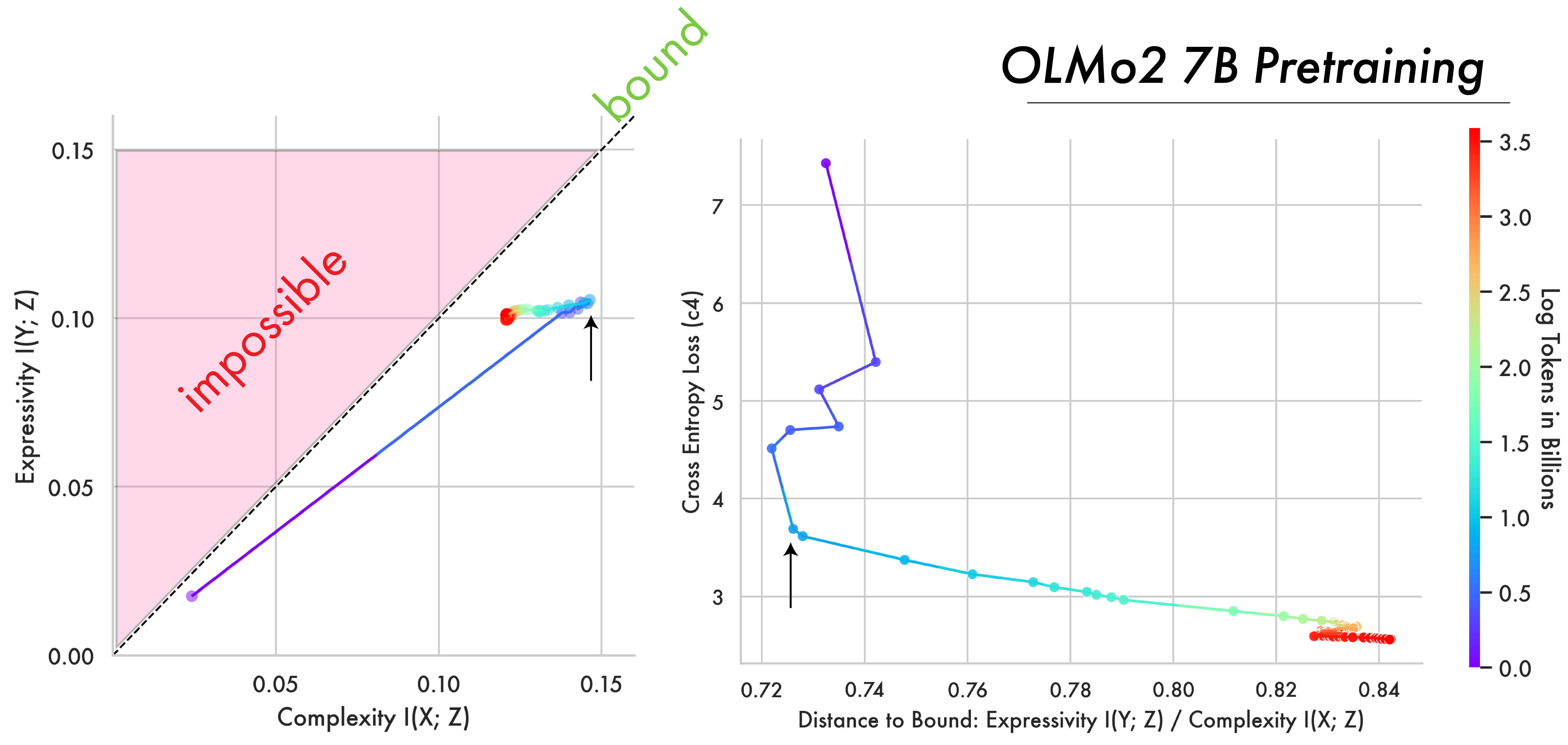
The majority of pre-training appears to be a slow compression of a model’s training data. The Information Bottleneck theory of deep learning predicts two phases: a fitting phase during which output information \(I(Y;Z)\) increases, followed by a compression phase during which input information \(I(X;Z)\) decreases and representations approach the bound. This transition to compression is believed to occur when error on the training set saturates.
Shown in the figure above is the training trajectory for the OLMo2 7B model with respect to data from English C4. Strikingly, the 7B model closely follows the two-phase prediction from the Information Bottleneck, first increasing mutual information with outputs, before compressing input information and progressing towards the bound on optimal compression. Additionally this transition appears to happen as the model’s loss on next-token prediction begins to saturate. This shows how, even at scale, deep-learning models appear to thread a needle between representational complexity and expressivity. It also demonstrates how LLMs can be effectively studied from the perspective of Rate Distortion Theory, as they try to converge to an optimal lossy compression of their training data.
Embeddings Largely Encode Local Context
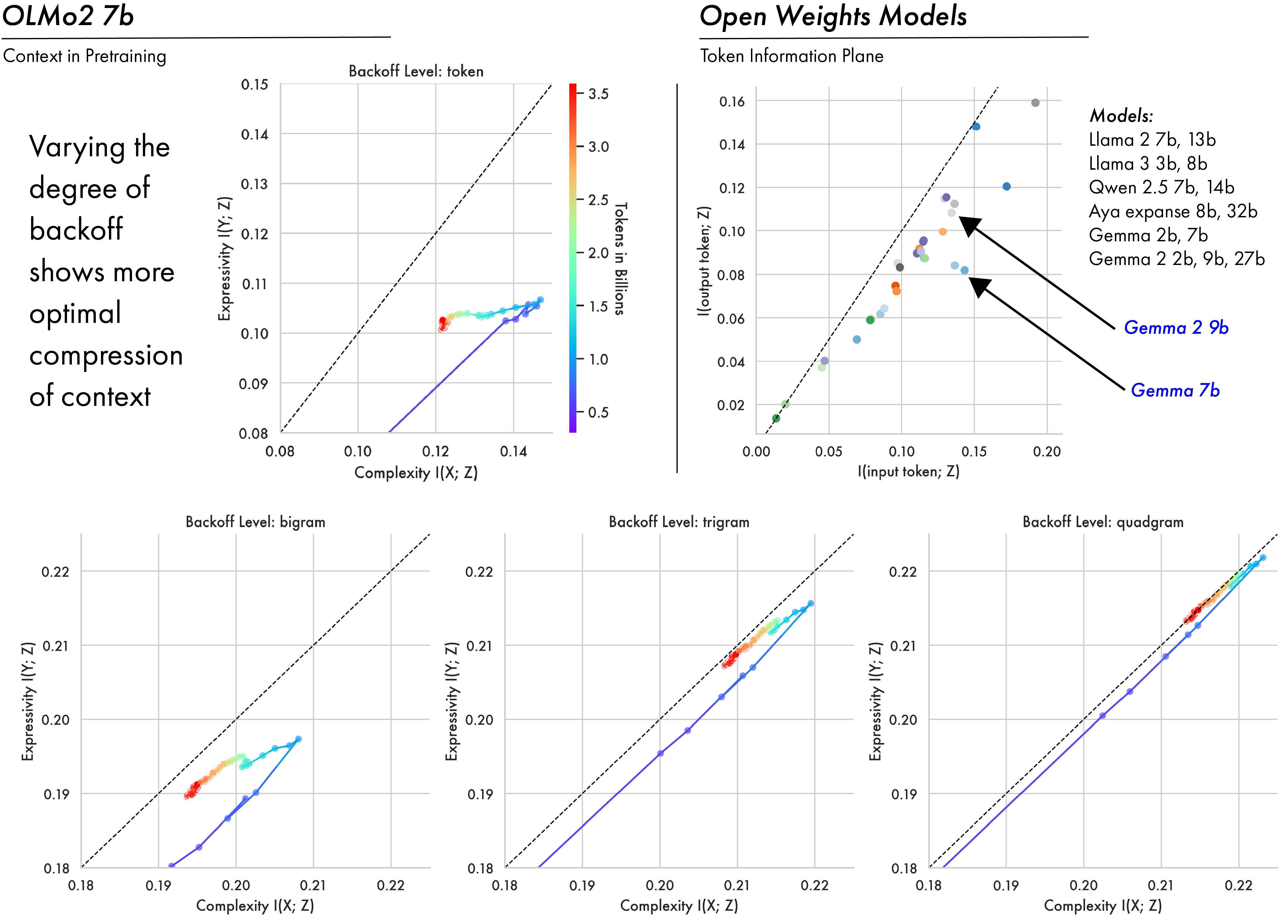
By varying the degree of backoff in the conditional distribution used to compute mutual information, we can see how contextual information evolves over pre-training at the token, bigram, trigram, and quad-gram levels. All cases result in a similar two-phase pattern of expansion and compression, with larger conditioning context converging closer to the bound. There is also a pattern of convergence where quad-grams account for only marginally more information than trigrams – suggesting representations largely encode local context, likely reflecting the information locality of the natural language on which they’re trained (Gibson 1998; Gibson et al. 2000; Hahn et al. 2022). This high degree of optimality in contextual encodings also likely reflects an inherent pressure in the pre-training objective for models to not only develop token representations, but representations of a token in context.

The Effect of Scale: Smaller Models Struggle to Compress
Parameter count shows a marked effect on the degree of compression achievable by a model. The figure above shows pre-training trajectories for the 1B, 7B, and 32B parameter models. The larger models both closely follow the hypothesized Information Bottleneck trajectory, exhibiting phases of expansion and compression, ultimately approaching optimal compression. The 1B parameter model exhibits markedly different behaviour. While it successfully completes the initial expansion phase – increasing output information \(I(Y;Z)\) – it fails to approach optimal compression. Instead, in the second phase the smaller model oscillates while moving slowly away from the theoretical frontier. Correlations between training step and complexity show larger models compress representations, with the 1B model significantly expanding. Correlations between step and the ratio of expressivity over complexity – which increases as models approach the bound – show only larger models consistently approach the bound (as indicated by positive correlation coefficients). This suggests that for a given level of data complexity, a certain parameter threshold may be necessary for models to achieve an optimal compression – an observation in line with work on scaling laws (Kaplan et al. 2020).
Convergence Patterns Across Open-Weight Models
In addition to looking at the OLMo2 family of models, we compute complexity and expressivity estimates across a diverse array of open-weight models (for tractability here we backoff to the token and bigram levels). A striking convergence pattern emerges: across different model families, hyperparameters, and training methodologies, representations ultimately converge to token and bigram informations clustered near the optimal bound on compression. This suggests that training as a process of compression is not an artifact of a single LLM’s training trajectory, but more fundamentally applies to to deep-learning models as a class, and to the data and the objectives used to train them.
Relating Representation Structure to Performance
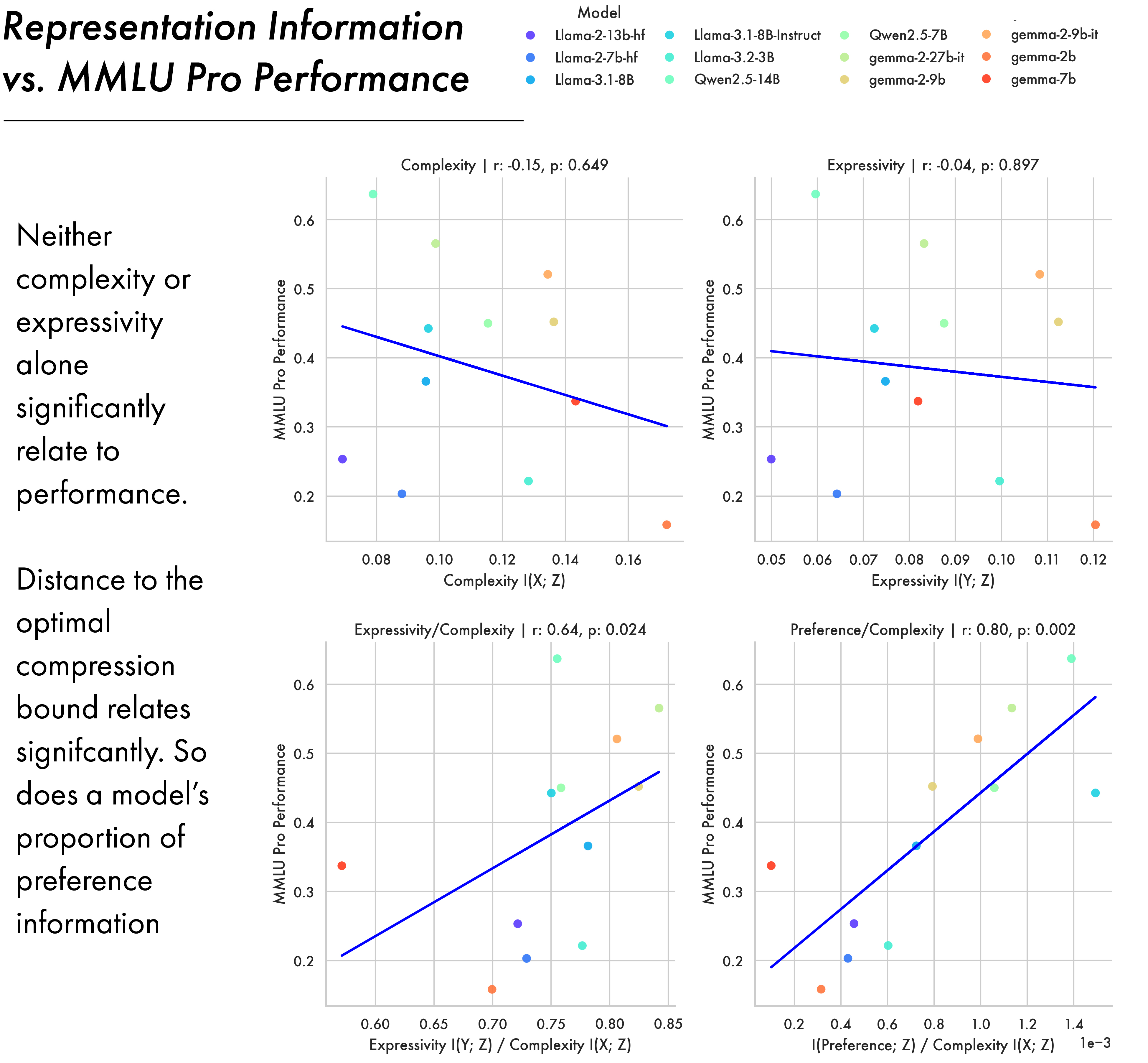
So far we have studied how information in an LLM is structured; we now consider how that structure relates to downstream performance. The figure above shows correlations between representational measures and performance on the MMLU Pro benchmark (Wang et al. 2024) for open weights models from 3 different families. Complexity alone proves not to be predictive of performance (\(r=-0.15\), \(p=0.649\)), neither does expressivity (\(r=-0.04\), \(p=0.897\)). However, the ratio between expressivity and complexity is a significant predictor (\(r=0.64\), \(p=0.024\)). This ratio indicates how close a model is to optimal compression, since it approaches 1.0 as the model approaches the IB bound. Together, these results indicate that compression alone is not a significant predictor of performance, but the optimality of that compression is.
While LLMs approach optimal compression for next sequence prediction over pre-training, a large body of work also tries to improve their ability to follow instructions, and generate responses humans prefer (Ouyang et al. 2022). We use preference data (Lambert et al. 2024) to compute mutual information with preference. As shown in the figure above, the ratio between a model’s complexity and the amount of preference information it contains also proves a significant predictor of downstream performance (\(r=0.8\), \(p=0.002\)). This suggests that not only does the optimality of a model’s compression matter, but exactly what information survives that compression does too.
These results also indicate how the information theoretic approach taken here could potentially be leveraged during training. Two applications could be as a stopping-criterion – ceasing pre-training when distance to the bound no longer decreases, or as a model-selection criterion – picking the checkpoint that is the most optimally compressed, or with the highest proportion of preference information. Given the estimates here are computed with a single-forward pass using teacher forcing, computing an entropy estimate for candidate selection would be substantively less costly than evaluating a model across a suite of benchmarks. We look to experimentally validate these potential use cases of our approach in future work.
Conclusion
The work presented here bridges the gap between theoretical accounts of learning and the practical complexities of LLMs. We show that LLMs learn an optimal compression of the data on which they are trained, with a wide array of open-weights models converging near the IB bound – with the optimality of a model’s compression predicting downstream performance. Each compression is different; we can account for the information that survives the compressive process, showing how representations encode information about different levels of local context and human preferences.
The approach to interpretability we introduce here interprets a model as a whole – rather than focussing on a particular circuit, or attention head – because complex distributed systems are not best understood in terms of their parts alone. Giving a holistic account of what it means to train an entire model on the entire internet is a challenge, but we argue that LLMs are best understood as lossy compression. In doing so, we place them in the context of a long history of work on representation learning across the sciences.